

In economic models of “learning-by-doing,” technological progress is an incidental outcome of production: the more a firm or worker does something, the better they get at it. In its stronger form, the idea is formalized as a “learning curve” (also sometimes called an experience curve or Wright’s Law), which asserts that every doubling of total experience leads to a consistent decline in per-unit production costs. For example, every doubling of the cumulative number of solar panels installed is associated with a 20% decline in their cost, as illustrated in the striking figure below (note both axes are in logs).

Learning curves have an important implication: if we want to lower the cost of a new technology, we should increase production. The implications for combating climate change are particularly important: learning curves imply we can make renewable energy cheap by scaling up currently existing technologies.
But are learning curves true? The linear relationship between log costs and log experience seems to be compelling evidence in their favor - it is exactly what learning-by-doing predicts. And similar log-linear relationships are observed in dozens of industries, suggesting learning-by-doing is a universal characteristic of the innovation process.
But what if we’re wrong?
But let’s suppose, for the sake of argument, the idea is completely wrong and there is actually no relationship between cost reductions and cumulative experience. Instead, let’s assume there is simply a steady exponential decline in the unit costs of solar panels: 20% every two years. This decline is driven by some other factor that has nothing to do with cumulative experience. It could be R&D conducted by the firms; it could be advances in basic science; it could be knowledge spillovers from other industries, etc. Whatever it is, let’s assume it leads to a steady 20% cost reduction every two years, no matter how much experience the industry has.
Let’s assume it’s 1976 and this industry is producing 0.2 MW every two years, and that total cumulative experience is 0.4 MW. This industry faces a demand curve - the lower the price, the higher the demand. Specifically, let’s assume every 20% reduction in the price leads to a doubling of demand. Lastly, let’s assume cost reductions are proportionally passed through to prices.
How does this industry evolve over time?
In 1978, cost and prices drop 20%, as they do every every two years. The decline in price leads demand to double to 0.4 MW over the next two years. Cumulative experience has doubled from 0.4 to 0.8 MW.
In 1980, cost and prices drop 20% again. The decline in price leads demand to double to 0.8 MW per decade. Cumulative experience has doubled from 0.8 MW to 1.6 MW.
In 1982… you get the point. Every two years, costs decline 20% and cumulative experience doubles. If we were to graph the results, we end up with the following:

In this industry, every time cumulative output doubles, costs fall 20%. The result is the same kind of log-linear relationship between cumulative experience and cost as would be predicted by a learning curve.
But in this case, the causality is reversed - it is price reductions that lead to increases in demand and production, not the other way around. Importantly, that means the policy implications from learning curves do not hold. If we want to lower the costs of renewable energy, scaling up production of existing technologies will not work.
This point goes well beyond the specific example I just devised. In any demand curve with a constant elasticity of demand, it can be shown constant exponential progress yields the same log-linear relationship predicted by a learning curve. And even when demand doesn’t have a constant elasticity of demand, you can frequently get something that looks pretty close to a log-linear relationship, especially if there is a bit of noise.
But ok; progress is probably not completely unrelated to experience. What if progress is actually a mix of learning curve effects and constant annual progress? Nordhaus (2014) models this situation, and also throws in growth of demand over time (which we might expect if the population and income are both rising). He shows you’ll still get a constant log-linear relationship between cost and cumulative experience, but now the slope of the line in such a figure is a mix of all these different factors.
In principle, there is a way to solve this problem. If progress happens both due to cumulative experience and due to the passage of time, then you can just run a regression where you include both time and total experience as explanatory variables for cost. To the extent experience varies differently from time, you can separately identify the relative contribution of each effect in a regression model. Voila!
But the trouble is precisely that, in actual data, experience does not tend to differ from time. Most markets tend to grow at a steady exponential rate, and even if they don’t, their cumulative output does. This point is made pretty starkly by Lafond et al. (2018), who analyze real data on 51 different products and technologies. For each case, they use a subset of the data to estimate one of two forecasting models: one based on learning curves, one based on constant annual progress. They then use the estimated model to forecast cost for the rest of the data and compare the accuracy of the methods. In the majority of cases, they tend to perform extremely similarly.
To take one illustrative example, the figure below forecasts solar panel costs out to 2024. Beginning in 2015 or so, the dashed line is their forecast and confidence interval for a model assuming constant technological progress (which they call Moore’s law). The red lines are their forecasts and confidence intervals for a model assuming learning-by-doing (which they call Wright’s law). The two forecasts are nearly identical.

So the main point, so far, is that consistent declines in cost whenever cumulative output doubles is not particularly strong evidence for learning curves. Progress could be 100% due to learning, 100% due to other factors, or any mix of the two, and you will tend to get a result that looks the same.
But that doesn’t mean learning curves are not true - only that we need to look for different evidence.
A theoretical case for learning curves
One reason I think learning curves are sort-of true is that they just match our intuitions about technology. We have a sense that young technologies make rapid advances and mature ones do not. This is well “explained” by learning curves. By definition, firms do not have much experience with young technologies; therefore it is relatively easy to double your experience. Progress is rapid. For mature technologies, firms have extensive experience, and therefore achieving a doubling of total historical output takes a long time. Progress is slow.
There is a bit of an issue of survivor bias here. Young technologies that do not succeed in lowering their costs never become mature technologies. They just become forgotten. So when we look around at the technologies in widespread use today, they tend to be ones that successfully reduced cost until they were cheap enough to find a mass market, at which point progress plateaued. All along the way, production also increased since demand rises when prices fall. (Even here, it’s possible to think of counter-examples: we’ve been growing corn for hundreds of years, yet yields go up pretty consistently decade on decade)
But even acknowledging survivor bias, I think learning-by-doing remains intuitive. Young technologies have a lot of things that can be improved. If there’s a bit of experimentation that goes alongside production, then many of those experiments will yield improvements simply because we haven’t tried many of them before. Mature technologies, on the other hand, have been optimized for so long that experimentation is rarely going to find an improvement that’s been missed all this time.
There’s even a theory paper that formalizes this idea. Auerswald, Kauffman, Lobo, and Shell (2000) apply models drawn from biological evolution to technological progress. In their model, production processes are represented abstractly as a list of subprocesses. Every one of these sub-processes has a productivity attached to it, drawn from a random distribution. The productivity of the entire technology (i.e., how much output the technology generates per worker) is just the sum of the productivities of all the sub-processes. For instance, in their baseline model, a technology has 100 sub-processes, each sub-process has a productivity ranging from 0 to 0.01, so that the productivity of the entire technology when you add them up ranges from 0 to 1.
In their paper, firms use these technologies to produce a fixed amount of output every period. This bypasses the problem highlighted in the previous section, where lower costs lead to increased production - here production is always the same each period, and is therefore unrelated to cost. As firms produce, they also do a bit of experimentation, changing one or more of their sub-processes at a constant rate. When changes result in an increase in overall productivity, the updated technology gets rolled out to the entire production process next period, and experimentation begins starting from this new point.
In this way, production “evolves” towards ever higher productivity and ever lower costs. What’s actually happening is that when a production process is “born” the productivity of all of its sub-processes are just drawn at random so they are all over the map: some high, some low, most average. If you choose a sub-process at random, in expectation it’s productivity will just be the mean of the random distribution, and so if you change it there is a 50:50 shot that the change will be for the better. So progress is fairly rapid at first.
But since you only keep changes that result in net improvements, the productivity of all the sub-processes gets pulled up as production proceeds. As the technology improves, it gets rarer and rarer that a change to a sub-process leads to an improvement. So tinkering with the production process yields an improvement less and less often. Eventually, you discover the best way to do every sub-process, and then there’s no more scope to improve.
But even though this model give you progress that gets harder over time, it actually does not generate a learning curve, where a doubling of cumulative output generates a constant proportional increase in productivity. Instead, you get something like the following figure:
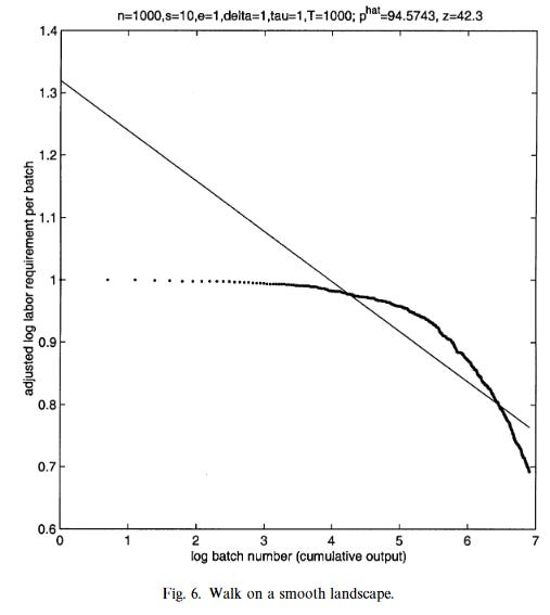
To get a figure that has a linear relationship between the log of cumulative output and the log of costs, the authors instead assume (realistically, in my view) that production is complex and sub-processes are interrelated. In their baseline model, every time you change one subprocess, the productivity of four other sub-processes is also redrawn.
In this kind of model, you do observe something like a learning curve. This seems to be because interdependence changes the rate of progress such that it speeds up in early stages and slows down in later ones. The rate of progress is faster at the outset, because every time you change one subprocess, you actually change the productivity of multiple subprocesses that interact with it. Since these changes are more likely to be improvements at the outset, that leads to faster progress when the technology is young, because you can change lots of things at once for the better.
But when a technology matures, the rate of progress slows. Suppose you have a fairly good production process, where most of the sub-processes have high productivity, but there are still some with low productivity. If you were to tinker with one of the low-productivity sub-processes, it’s pretty likely you’ll discover an improvement. But, you can’t just tinker with that one. If you make a change to the one, it will also lead to a change in several other sub-processes. And most of those are likely to be high-productivity. Which means any gains you make on the low-productivity sub-process will probably be offset by declines in the productivity of other ones with which it interacts.
When you add in these interdependencies between sub-processes, their model generates figures like the following. For much of their life, they look quite a lot like learning curves. (And remember, this is generated with constant demand every period, regardless of cost)

What’s encouraging is the story Auerswald, Kauffman, Lobo, and Shell are telling is one that sounds quite applicable to many real technologies. In lots of technologies there are many sub-components or sub-processes that can be changed, changes may result in improvements or deterioration, and changing one thing frequently affects other sub-components. If you go about this kind of randomly, you can get something that looks like a learning curve.
Evidence from an auto plant
Another paper by Levitt, List, and Syverson (2013) use a wealth of data from an automobile assembly plant to document exactly the kind of learning from experience and experimentation that undergirds learning curves. The paper follows the first year of operation for an auto assembly plant at an unnamed major automaker. Their observations begin after several major changes: the plant went through a major redesign, the firm introduced a new team-based production process, and the vehicle model platform had its first major redesign in six years. Rather than focus on the cost of assembling a car, the paper measures the decline in production defects as production ramps up.
Levitt, List, and Syverson observe a rapid reduction in the number of defects at first, when production is still in early days, followed by a slower rate of decline as production ramps up. Consistent with the learning curve model, the relationship between the log of the defect rate and the log of cumulative production is linear.

Learning-by-doing really makes sense in this context. Levitt, List and Syverson provide some concrete examples of what exactly is being learned in the production process. In one instance, two adjacent components occasionally did not fit together well. As workers and auditors noticed this, they tracked the problem to high variance in the shape of one molded component. By slightly adjusting the chemical composition of the plastic fed into the mold, this variability was eliminated and the problem solved. In another instance, an interior part was sometimes not bolted down sufficiently. In this case, the problem was solved by modifying the assembly procedure for those particular line workers, and adding an additional step for other workers to check the bolt. It seems reasonable to think of these changes as being analogous to changing subprocesses, each of which can be potentially improved and where changes in one process may affect the efficacy of others.
Levitt, List, and Syverson also show that this learning becomes embodied in the firm’s procedures, rather than the skill sets of the individual workers. Midyear, the plant began running a second line and on the second line’s first full day (after a week of training), their defect rate was identical to the first shift workers.

This is a particularly nice context to study because there were no major changes to the plant’s production technology during the period under review. There were not newly designed industrial robots installed midway through the year, or scientific breakthroughs that allowed the workers to be more efficient. It really does seem like, what changed over the year was the plant learned to optimize a fixed production technology.
An Experiment
So we have a bit of theory that shows how learning curves can arise, and we’ve got one detailed case study that seems to match up with the theory pretty well. But it would be really nice if we had experimental data. If we were going to test the learning curve model and we had unlimited resources, the ideal experiment would be to pick a bunch of technologies at random and massively ramp up their production, and then to compare the evolution of their costs to a control set. Better yet, we would ramp up production at different rates, and in a way uncorrelated with time, for example, raising production by a lot but then shutting it down to a trickle in later years. This would give us the variation between time and experience that we need to separately identify the contribution to progress from learning and from other stuff that is correlated with the passage of time. We don’t have that experiment, unfortunately. But we do have World War II.
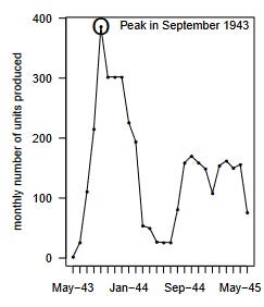
The US experience in World War II is not a bad approximation of this ideal experiment. The changes in production induced by the war were enormous: the US went from fielding an army of under 200,000 in 1939 to more than 8 million in 1945, and also equipping the allied nations more generally. The production needs were driven by military exigencies more than the price and cost of production, which should minimize reverse causality, where cost declines lead to production increases. Production was also highly variable, so that it is possible to separately identify cost reductions associated with time and cumulative experience. The following figure, for example, illustrates monthly production of Ford’s Armored Car M-20 GBK.
A working paper by Lafond, Greenwald, and Farmer (2020) uses this context to separately identify wartime cost reductions associated with production experience and those associated with time. They use three main datasets:
Man hours per unit over the course of the war for 152 different vehicles (mostly aircraft, but also some ships and motor vehicles)
Total unit costs per product for 523 different products (though with only two observations per product: “early” cost and “later” costs)
Indices of contract prices aggregated up the level of 10 different war sub departments
So, in this unique context, we should be able to accurately separate out the effect of learning-by-doing from other things that reduce cost and are correlated with the passage of time. When Lafond, Greenwald, and Farmer do this, they find that cost reductions associated specifically with experience account for 67% of the reduction in man hours, 40% of the reduction in total unit costs, and 46% of the reduction in their index of contract prices. Learning by doing, at least in World War II, was indeed a significant contributor to cost reductions.
Are learning curves useful?
So where do stand, after all that? I think we have good reason to believe that learning-by-doing is a real phenomenon, roughly corresponding to a kind of evolutionary process. At the same time, it almost certainly accounts for only part of the cost reductions we see in any given project, especially over the long-term when there are large changes to production processes. In particular, the historical relationship between cost reductions and cumulative output that we observe in “normal” circumstances is so hopelessly confounded that we really can’t figure out what share accrues to learning-by-doing and what share to other factors.
That means that if we want to lower the costs of renewable energy (or any other new technology), we can probably be confident they will fall to some degree if we just scale up production of the current technology. But we don’t really know how much - historic relationships don’t tell us much. In World War II, at best, we would have gotten about two-thirds of the rate of progress implied by the headline relationship between cost reduction and cumulative output. Other datasets imply something closer to two fifths. Moreover, the evidence reviewed here applies best to situations where we have a standard production process around which we can tinker and iterate to a higher efficiency. If we need to completely change the method of manufacture or the structure of the technology - well, I don’t think we should count on learning by doing to deliver that.
The next newsletter (January 19) will be about the challenges in getting any academic field to embrace new (better) methodologies, and how the field of economics overcame them.
If you enjoyed this post, you might also enjoy:


